Results¶

At the end of the run, proj-0/systems/final-results/ contains:

final.gro, final.top, final.tpx, final.grx — the cured polystyrene system in GROMACS-friendly form;
final.viz.psf, final.viz.tcl — VMD-friendly companion files that carry the real bond topology and trim PBC-crossing bonds at display time. Open with:
```
$ vmd final.viz.psf final.gro -e final.viz.tcl
```

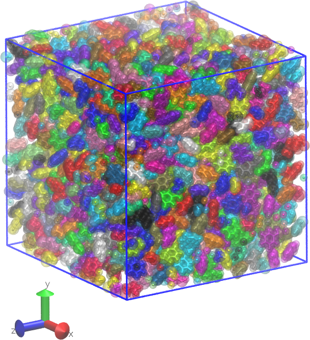
../../_images/final-box.png — Fig. 10 The cured polystyrene box rendered from `final.viz.psf` + `final.gro`. The TCL helper has trimmed bonds that would otherwise wrap across the periodic image, leaving each polymer chain visually contiguous.¶

Plots from the build log¶

htpolynet writes per-stage trace plots into proj-0/plots/ and a machine-readable proj-0/profile.json recording wall time per stage and subprocess time per tool. The plotting subcommand can also produce summary figures from the diagnostic log:

$ htpolynet plots -diag diagnostics.log

A further exercise¶

Copy the YAML and dial down the desired conversion to see what the same cure looks like at a lower extent of reaction:

$ cp 1-polystyrene.yaml 1-polystyrene-low.yaml
$ # edit 1-polystyrene-low.yaml: CURE.controls.desired_conversion: 0.50
$ htpolynet run -diag diagnostics-low.log 1-polystyrene-low.yaml &> console-low.log &

The second build lands in proj-1/. Comparing density traces and the profile.json files between the two runs gives a feel for how much of the total wall time goes into the cure loop itself.

Post-build analyses¶

Once you have a cured polystyrene system, htpolynet postsim and htpolynet analyze can drive production MD and compute properties such as the glass-transition temperature. See the Post-build simulations and analyses section for the recommended workflow for this system; DGEBA-PACM Epoxy Thermoset shows the full set of techniques (including uniaxial deformation for Young’s modulus) with real production-quality plots.